

Saturday Speculations #1: Expectations Investing
Saturday Speculations #1: Expectations Investing
“In every chain of reasoning, the evidence of the last conclusion can be no greater than that of the weakest link of the chain, whatever may be the strength of the rest.” ~Thomas Reid

I hope you all enjoyed the activist pitch on TARO 0.00%↑ ! I’ll share an update on that next month; some interesting new developments with Sun (ParentCo) facing a shortage of working capital to cover commitments.
I’m working on another name that was a spin from a $100b+ company. The company has been engaged in litigation against its parent, resolved in late 2020 during a bankruptcy event. Since then, it’s been saddled with preferred shares accruing at 11% - and only a sale allows for early redemption. Dynamics heavily favor an acquisition, and the company was reportedly shopping for options in November.
Expectations Investing
Last week, I worked again on an ‘expectations investing’ exercise that I first ran on XOM 0.00%↑ during the 2020 COVID decline (wish I had put more into that trade!). I was reminded of how great the exercise is - and also how it’s so internalized for that reframing the investment question explicitly offers a lot of clarity. It’s particularly relevant now in a post-COVID environment.
When I first ran the exercise, I’d never read Expectations Investing by Mauboussin and Rappaport.
Instead, I was building on a simple realization:
“If I’m modelling, I make certain assumptions to get to an implied price for an equity. Well, the market already gives me a price, so what if I just build a reverse-DCF?”
-Younger me, reinventing the wheel
This was groundbreaking for me as a beginning investor. Below, I’ll talk about what I learned, the traps I fell into, and how this shaped my investment philosophy. I rather appreciate that it took me a while to get around to reading Expectations Investing - it makes my initial view a little more ‘pure’ somehow.
First Pass: XOM and multiple arbitrage
I’m sure you all remember March 2020 - and the massive opportunities that decline presented. I found myself pitching Exxon right after the decline, around $52. The red charts below are from that pitch deck.

My first approach to this exercise was a bit misguided. I began with a complete DCF for XOM, and wrote a basic VBA macro that automatically solved for the exit multiple that made the implied stock price equal the current stock price. Implicit in using the multiple to model the current stock price is me assuming that...
…all of my business assumptions (IS/BS/CFS) match the market exactly.
…my WACC assumption is accurate and is the cost of capital that all other investors have assumed.
…XOM has a ‘true’ future market multiple that I can compare my derived multiple with.
Essentially, I assumed that my model was perfectly market expectations - and the only source of price variation in the market was investors’ market multiple vs. the theoretical ‘true’ XOM multiple. If I knew those numbers, I could arbitrage that.
That was a mistake.
I had relied on analyst estimates, well-covered data, and things that were definitely priced in. What I couldn’t price anything sell-side couldn’t tell me. As I’m sure you know, sell-side analysts tend to disagree quite a bit and it’s an exercise in futility to find a real consensus.
But I got my 0% return!

Let’s compare the output above to what actually happened.
I had XOM’s 2025 EBITDA estimate at $45b for 2025E. It’s on track to make $100b this year alone, and will normalize to $75b by 2025, 50% above my estimates.
I had XOM’s derived multiple at 6.5x - it traded at a lot higher than that through 2020 and 2021.
It could have been timed better - XOM dropped down to $32 after this pitch before surging. That implied a multiple of only 4.5x NTM EBITDA! XOM still trades above that.
Exxon is still over double the price it was pitched at. It’s a great outcome, sure - but the modeling exercise didn’t really contribute much besides confirm that it was cheap at the current price. There wasn’t any expectations valuation yet.
Making Mistakes: Bear Case
The XOM modeling experience still heavily changed my process. I started modelling bear cases almost exclusively. Not true bear cases - just rough economic environments. I would say things like:
“To get a bear case - where we only make the cost of capital - we’d need to assume 500bps lower FCF margin and a 2-turns lower multiple. That situation only happens if we have an ‘08/’09 level recession.”
-Still younger me, making new mistakes
If I trust your work, the statement above is very convincing to me. And so as I modeled, my cases would be unrealistically conservative. Anything someone would raise as a risk was generally already modeled in pretty aggressively.
I’ve since learned that people always like to add a margin of safety of their own, regardless of how safe your projections are. They’d take my safe case, haircut the margins more, and be shocked that the model wasn’t bullish anymore.
That does explain why I had such a low pitch hit rate that year…

This isn’t an indictment of bearish modeling. For me, the ideal expectations investing model is still bearish. It might not be true, but the determination you need as an investor is just: “Will this stock meet my hurdle rate? What would I have to assume for the business to justify the current stock price?
Refining the Process: The Current Version
All this brings us to present day, when I found myself building an evolved version of the same model.
I won’t name the company, but it’s a large business that earns revenue at industry growth (1%) + pricing growth (2%). Revenue growth in excess of 3%, or under, is typically market share gain or loss. Given the nature of the business, I can confidently say my margin, multiple, and WACC assumptions are pretty accurate.
The big uncertainty here is revenue - in a post-COVID world, will the industry grow at the same rate as before? Will pandemic revenue gains be the new baseline, or is 2023 going to be a revenue correction before we return to steady growth?
Below are two revenue examples - one where we see pandemic over-earning, and one that’s steady state growth.
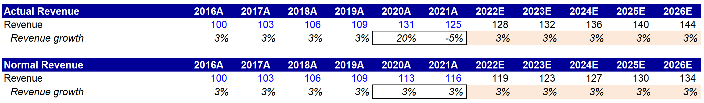
As you can see, in the ‘actual’ revenue model, the pandemic bump drives overearning through the entire projection period. With constant margin assumptions, the ‘actual’ model benefits from greater investment period cash flows and a higher exit multiple valuation.
Now, you can’t just ignore the true financials. However, you can figure out which purchase price makes what revenue assumption out until 2026. The statement we’re looking to answer is:
“At a $__ purchase price, you are assuming __% annual revenue growth through 2026 to achieve a 4 year double*. This represents a revenue CAGR of __% from 2019 to 2026.”
*4 year double is also an assumption! Replace this with whatever your return target is; maybe a five year triple, etc.
Output and Walkthrough

Let’s walk through it step by step. If this stock is priced at $56, I would need to believe in 2.5% revenue growth from 2023-2026 to meet my 4 year double hurdle rate. This implies growth of 2.9% from 2019-2026.
The 2019-2026 number is a sanity check. Using 2019 as a base year, I want to be sure that I’m not implicitly assuming above-3% growth rates through the projection period.
Now, if I’m comfortable with a 3% revenue assumption, I should be willing to buy at $56 and below. At $56, I’m comfortable buying in. At $53, I’m sizing up. At $50, ceteris paribus, I’m buying all I can get my hands on.
That’s not to say the business can’t grow above 3%; but that 3% is the upper bound growth that I am comfortable underwriting. Maybe someone else prefers 2.6% as steady state growth - their price would be $55.
I now know exactly when to buy and sell.
Considerations
The model is a two way street. When I ask “What rate of revenue growth justifies a $10 stock price?” I can also ask “At a $10 stock price, what rate of revenue growth would I need to believe to be a buyer?”
By only modelling for revenue growth, you’re implicitly assuming that your other assumptions are correct. It’s possible to have multiple variables, but then it turns into a set of equations with multiple solutions. In that case, you have to go Monte Carlo.
Modifications
There’s a few different ways to make this calculation, and a lot of potential nuance you can add to make it fit your model. If you keep variable relationships linear, you can use data tables to solve. If you have circularity, then VBA is the only efficient method to solve. Any first year analyst should be able to figure out the data table method.
You could assume a certain percentage of pricing gains are kept in excess of 3%, or some additional market share gain.
You could run this directly on a normalized FCF or EBITDA basis if you don’t want to make explicit margin assumptions.
You can add a 1-2 year recession by projecting the ‘severity under the baseline’ growth detractor.
Say it’s a cyclical business - you can project the over/under of cyclicality each year/quarter, and solve for the baseline growth rate assumed.
You could run a Monte Carlo with your margin assumptions and revenue assumptions to really stress test it.
As always, make the model your own.
Conclusion
If you made it this far, I’m impressed. This writeup is mainly to organize my own thoughts on the topic, but I highly recommend trying it out. Coming out of COVID, understanding potential growth in a normalized environment is more important than ever.
I’m happy to talk more about this and different implementations I’ve done separately. It takes a bit of effort to get this really working, but getting the intuition right is the most important part.
Welcome back to earnings season - best of luck!
Onwards and upwards.